Response of a damped mass spring system excited by various conditions on...
In this
video, we will see how to find the response of a damped mass spring system
excited by various conditions.
Where m is
the mass, c the viscous damping coefficient and k the spring stiffness.
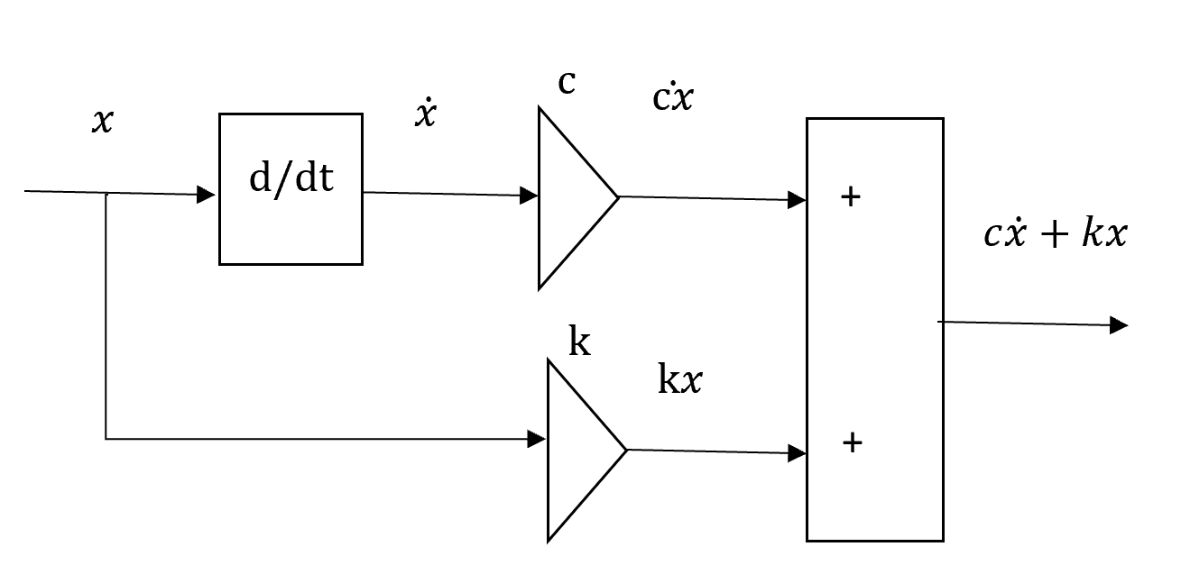
Using various
blocks, we will build our model piece by piece. From a function x, we get dx/dt by differentiating
with respect to time. Then we multiply dx/dt by c and x by k and sum the two expressions.
Adding the
external force and subtracting cdx/dt+kx then dividing by m we should get the
acceleration d2x/dt^2 which is also the result of differentiating dx/dt with respect to time
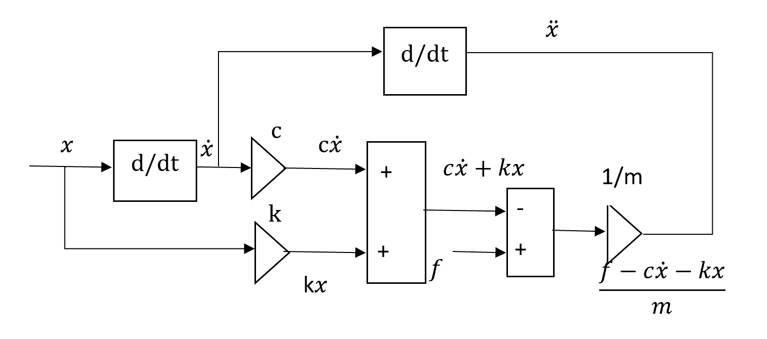
Working
with integrators is better than with differentiator as in the former we could
use the initial condition which gives better control on the solution obtained.
The model becomes:

On Simulink, we will need the following blocks: two integrators, 3 amplifiers, one constant, one oscilloscope and two blocks to calculate the sum of inputs

The blocks
are wired together to give the following model

In fact,
the two sum blocks could be merged into one block with 3 inputs and one output.
The number of inputs is the number of + and – signs

If we need
to recover one of the parameters in Matlab’s workspace, we could send it to the
workspace using the block ToWokspace

An object
out will be created with two components which are of interest here out.tout is
the simulation time and out.x which contains the solution x(t)
Now, let us
see what the transient solution is found by Simulink. Obviously, the mass
should not be at rest at t=0. Here we choose v0=1.
The
solution of the undamped system displayed on the oscilloscope is

If we
introduce damping, c=2

Of course,
the same plot is obtained if we plot out.x against out.tout
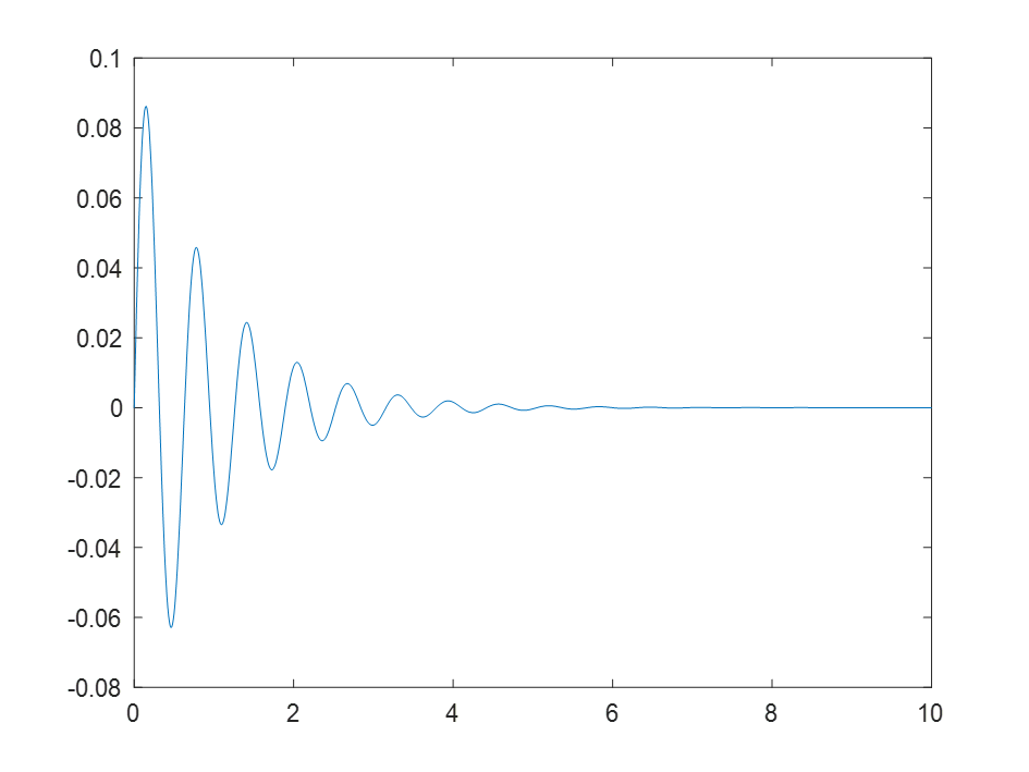

Notice that
0.1 corresponds to F/k=10/100
Now we will
consider a variable force. Let start with a sinusoidal force
We change
the constant force in the previous model with a sine source. Also, on the
oscilloscope, in addition to the response we display the force

The
amplitude is 10 and the excitation frequency is 10 rad/s without phase.

The
oscillations at the beginning are the manifestation of the transient behavior.
Part of it is due to the initial condition v0=1. After imposing zero initial
conditions, we obtain

Most of the
transient response has disappeared
Let’s move
to a different force, namely the step function. The force appears suddenly at
the step time (here 1 s) and remains constant (here 10)

The mass m,
initially at rest, remains so until the force appears. Then oscillates around
f/k=0.1

Instead of looking
for other sources individually or combine some sources to produce special
forces, we could use a signal generator which can generate a sine, a square, a
sawtooth or random signals.

The
response of the system when excited with a square force for instance is

Another interesting
source in Simulink is the waveform generator. It enables to define analytically
multiple signal expressions and choose one expression as output at a time.

Here we
create to signals one of expression sin(10,1,0)+.5*sin(10,2,0) we sum two
sinewaves one of amplitude 10 and frequency 1 rad/s and the second of amplitude
5 and frequency 2 rad/s.
The second
signal is the previous plus a pulse of amplitude 10 which starts at t=2s and
lasts for 3 s.
The chosen output
is the first expression

To improve the
smoothness of the input force we change the sampling frequency


The result
is much better

Now, from
our waveform generator, let’s change the out signal to the second expression


We get the
response of the system to a combination of two sine waves and one pulse
BTW, to
appreciate the usefulness and practicality of the wave generator, to generate
the same force we need four sources and a block to do the sum

The first
two generate sinewaves of 1 and 2 rad/s. The third source is a step function of
amplitude 10 and starts at t=2s and finally the fourth source is step function
of amplitude -10 and starts at t=5s (2s+duration of 3s).
Other
sources exist in Simulink, but we have seen the main ones. You are advised to
start using Simulink and discover all its capabilities.
Video on Youtube


Commentaires